Kernel Guide

Download this notebook: constructing_new_kernels.ipynb

In this guide, we introduce the kernels available in GPJax and demonstrate how to create custom kernels. We assume you already know what a kernel is and what it does to a GP prior; if not, our introduction to kernels builds that intuition first.

# Enable Float64 for more stable matrix inversions.
from utils import use_mpl_style
from gpjax.kernels.base import _val
from gpjax.kernels.computations import DenseKernelComputation
from gpjax.parameters import PositiveReal
from jax import config
from jax.nn import softplus
import jax.numpy as jnp
import jax.random as jr
from jaxtyping import (
    Array,
    Float,
    install_import_hook,
)
import matplotlib.pyplot as plt

config.update("jax_enable_x64", True)


with install_import_hook("gpjax", "beartype.beartype"):
    import gpjax as gpx


# set the default style for plotting
use_mpl_style()

key = jr.key(42)

cols = plt.rcParams["axes.prop_cycle"].by_key()["color"]

Supported Kernels

The following kernels are natively supported in GPJax.

• Matérn 1/2, 3/2 and 5/2.

• RBF (or squared exponential).

• Rational quadratic.

• Powered exponential.

• Polynomial.

• White noise

• Linear.

• Polynomial.

• Graph kernels.

Whilst the syntax is consistent, each kernel’s type influences the characteristics of the sample paths drawn. We visualise this in Fig. 40 with 10 function draws per kernel.

kernels = [
    gpx.kernels.Matern12(),
    gpx.kernels.Matern32(),
    gpx.kernels.Matern52(),
    gpx.kernels.RBF(),
    gpx.kernels.Polynomial(),
    gpx.kernels.Polynomial(degree=2),
]
fig, axes = plt.subplots(ncols=3, nrows=2, figsize=(10, 6), tight_layout=True)

x = jnp.linspace(-3.0, 3.0, num=200).reshape(-1, 1)

meanf = gpx.mean_functions.Zero()

for k, ax, c in zip(kernels, axes.ravel(), cols, strict=False):
    prior = gpx.gps.Prior(mean_function=meanf, kernel=k)
    rv = prior(x)
    y = rv.sample(key=jr.key(22), sample_shape=(10,))
    ax.plot(x, y.T, alpha=0.7, color=c)
    ax.set_title(type(k).__name__)

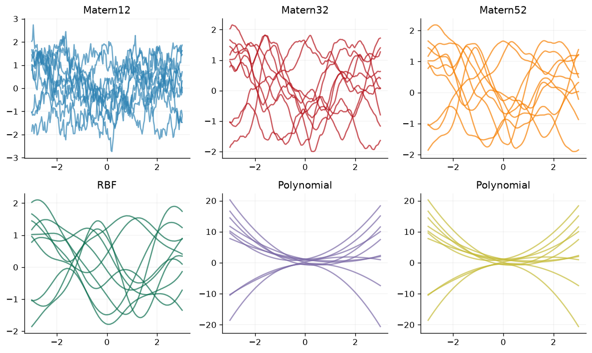
Fig. 40 Ten prior function draws for each of six natively supported kernels, showing how the choice of kernel controls the smoothness and shape of the sample paths.

Active dimensions

By default, kernels operate over every dimension of the supplied inputs. In some use cases, it is desirable to restrict kernels to specific dimensions of the input data. We can achieve this by the active dims argument, which determines which input index values the kernel evaluates.

To see this, consider the following 5-dimensional dataset for which we would like our RBF kernel to act on the first, second and fourth dimensions.

slice_kernel = gpx.kernels.RBF(active_dims=[0, 1, 3], lengthscale=jnp.ones((3,)))

The resulting kernel has one length-scale parameter per input dimension - an ARD kernel.

print(f"Lengthscales: {slice_kernel.lengthscale}")

Lengthscales: PositiveReal(_unconstrained=f64[3])

We’ll now simulate some data and evaluate the kernel on the previously selected input dimensions.

# Inputs
x_matrix = jr.normal(key, shape=(50, 5))

# Compute the Gram matrix
K = slice_kernel.gram(x_matrix).as_matrix()
print(K.shape)

(50, 50)

Kernel combinations

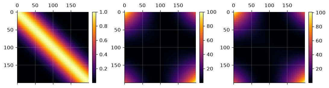
The product or sum of two positive definite matrices yields a positive definite matrix. Consequently, summing or multiplying sets of kernels is a valid operation that can give rich kernel functions. In GPJax, functionality for a sum kernel is provided by the SumKernel class.

k1 = gpx.kernels.RBF()
k2 = gpx.kernels.Polynomial()
sum_k = gpx.kernels.SumKernel(kernels=[k1, k2])

fig, ax = plt.subplots(ncols=3, figsize=(9, 3))
im0 = ax[0].matshow(k1.gram(x).as_matrix())
im1 = ax[1].matshow(k2.gram(x).as_matrix())
im2 = ax[2].matshow(sum_k.gram(x).as_matrix())

fig.colorbar(im0, ax=ax[0], fraction=0.05)
fig.colorbar(im1, ax=ax[1], fraction=0.05)
fig.colorbar(im2, ax=ax[2], fraction=0.05)

<matplotlib.colorbar.Colorbar at 0x7f7ddcd6b950>

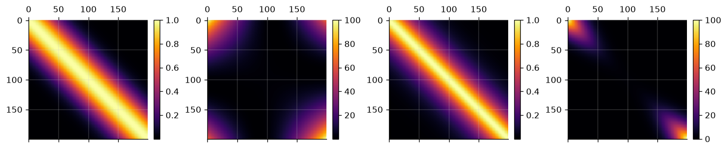
Similarly, products of kernels can be created through the ProductKernel class.

k3 = gpx.kernels.Matern32()

prod_k = gpx.kernels.ProductKernel(kernels=[k1, k2, k3])

fig, ax = plt.subplots(ncols=4, figsize=(12, 3))
im0 = ax[0].matshow(k1.gram(x).as_matrix())
im1 = ax[1].matshow(k2.gram(x).as_matrix())
im2 = ax[2].matshow(k3.gram(x).as_matrix())
im3 = ax[3].matshow(prod_k.gram(x).as_matrix())

fig.colorbar(im0, ax=ax[0], fraction=0.05)
fig.colorbar(im1, ax=ax[1], fraction=0.05)
fig.colorbar(im2, ax=ax[2], fraction=0.05)
fig.colorbar(im3, ax=ax[3], fraction=0.05)

<matplotlib.colorbar.Colorbar at 0x7f7ddcbfc650>

Custom kernel

GPJax makes the process of implementing kernels of your choice straightforward with two key steps:

1. Listing the kernel’s parameters.

2. Defining the kernel’s pairwise operation.

We’ll demonstrate this process now for a circular kernel - an adaption of the excellent guide given in the PYMC3 documentation. We encourage curious readers to visit their notebook here.

Circular kernel

When the underlying space is polar, typical Euclidean kernels such as Matérn kernels are insufficient at the boundary where discontinuities will present themselves. This is due to the fact that for a polar space \(\lvert 0, 2\pi\rvert=0\) i.e., the space wraps. Euclidean kernels have no mechanism in them to represent this logic and will instead treat \(0\) and \(2\pi\) and elements far apart. Circular kernels do not exhibit this behaviour and instead wrap around the boundary points to create a smooth function. Such a kernel was given in Padonou & Roustant (2015) where any two angles \(\theta\) and \(\theta'\) are written as

(1)\[ \begin{aligned} W_c(\theta, \theta') & = \left\lvert \left(1 + \tau \frac{d(\theta, \theta')}{c} \right) \left(1 - \frac{d(\theta, \theta')}{c} \right)^{\tau} \right\rvert \quad \tau \geq 4. \end{aligned} \]

Here the hyperparameter \(\tau\) is analogous to a lengthscale for Euclidean stationary kernels, controlling the correlation between pairs of observations. Whilst \(d\) is an angular distance metric

(2)\[ d(\theta, \theta') = \lvert (\theta-\theta'+c) \operatorname{mod} 2c - c \rvert. \]

To implement this, one must write the following class.

def angular_distance(x, y, c):
    return jnp.abs((x - y + c) % (c * 2) - c)


class Polar(gpx.kernels.AbstractKernel):
    period: float
    tau: PositiveReal

    def __init__(
        self,
        tau: float = 5.0,
        period: float = 2 * jnp.pi,
        active_dims: list[int] | slice | None = None,
        n_dims: int | None = None,
    ):
        super().__init__(active_dims, n_dims, DenseKernelComputation())
        self.period = jnp.array(period)
        self.tau = PositiveReal(jnp.array(tau - 4.0))

    def __call__(
        self, x: Float[Array, "1 D"], y: Float[Array, "1 D"]
    ) -> Float[Array, "1"]:
        c = self.period / 2.0
        t = angular_distance(x, y, c)
        tau = 4.0 + _val(self.tau)
        K = (1 + tau * t / c) * jnp.clip(1 - t / c, 0, jnp.inf) ** tau
        return K.squeeze()

We unpack this now to make better sense of it. In the kernel’s initialiser we specify the length of a single period. As the underlying domain is a circle, this is \(2\pi\). We then define the kernel’s __call__ function which is a direct implementation of Eq. 1 where we define c as half the value of period.

To constrain \(\tau \geq 4\), we store \(\tau - 4\) as a PositiveReal (which applies softplus internally) and add 4 back in __call__. The backend guide covers the parameter types available for declaring a parameter’s support in this way.

Using our polar kernel

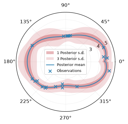
We proceed to fit a GP with our custom circular kernel to a random sequence of points on a circle (see the Regression notebook for further details on this process).

# Simulate data
angles = jnp.linspace(0, 2 * jnp.pi, num=200).reshape(-1, 1)
n = 20
noise = 0.2

X = jnp.sort(jr.uniform(key, minval=0.0, maxval=jnp.pi * 2, shape=(n, 1)), axis=0)
y = 4 + jnp.cos(2 * X) + jr.normal(key, shape=X.shape) * noise

D = gpx.Dataset(X=X, y=y)

# Define polar Gaussian process
PKern = Polar()
meanf = gpx.mean_functions.Zero()
likelihood = gpx.likelihoods.Gaussian(num_datapoints=n)
circular_posterior = gpx.gps.Prior(mean_function=meanf, kernel=PKern) * likelihood

# Optimise GP's marginal log-likelihood using BFGS
opt_posterior, history = gpx.fit_scipy(
    model=circular_posterior,
    objective=lambda p, d: -gpx.objectives.conjugate_mll(p, d),
    train_data=D,
)

Optimization terminated successfully.
         Current function value: 30.902421
         Iterations: 22
         Function evaluations: 26
         Gradient evaluations: 26

Prediction

We’ll now query the GP’s predictive posterior at linearly spaced novel inputs and illustrate the results.

posterior_rv = opt_posterior.likelihood(opt_posterior.predict(angles, train_data=D))
mu = posterior_rv.mean
one_sigma = jnp.sqrt(posterior_rv.variance)

fig = plt.figure(figsize=(7, 3.5))
gridspec = fig.add_gridspec(1, 1)
ax = plt.subplot(gridspec[0], polar=True)

ax.fill_between(
    angles.squeeze(),
    mu - one_sigma,
    mu + one_sigma,
    alpha=0.3,
    label=r"1 Posterior s.d.",
    color=cols[1],
    lw=0,
)
ax.fill_between(
    angles.squeeze(),
    mu - 3 * one_sigma,
    mu + 3 * one_sigma,
    alpha=0.15,
    label=r"3 Posterior s.d.",
    color=cols[1],
    lw=0,
)
ax.plot(angles, mu, label="Posterior mean")
ax.scatter(D.X, D.y, alpha=1, label="Observations")
ax.legend()

<matplotlib.legend.Legend at 0x7f7dd7e79c90>

System configuration

%reload_ext watermark
%watermark -n -u -v -iv -w -a 'Thomas Pinder'

Author: Thomas Pinder

Last updated: Sat, 01 Aug 2026

Python implementation: CPython
Python version       : 3.11.15
IPython version      : 9.15.0

gpjax     : 0.18.0
jax       : 0.10.2
jaxtyping : 0.3.11
matplotlib: 3.11.1

Watermark: 2.6.0