Graph Kernels

Download this notebook: graph_kernels.ipynb

This notebook demonstrates how regression models can be constructed on the vertices of a graph using a Gaussian process with a Matérn kernel presented in Borovitskiy et al. [2021]. For a general discussion of the kernels supported within GPJax, see the kernels notebook.

import random

from utils import use_mpl_style

# Enable Float64 for more stable matrix inversions.
from jax import config
import jax.numpy as jnp
import jax.random as jr
from jaxtyping import install_import_hook
import matplotlib as mpl
import matplotlib.pyplot as plt
try:
    from myst_nb import glue
except ImportError:  # notebook downloaded and run outside the docs build
    def glue(*args, **kwargs):
        """No-op stand-in: gluing only matters when Sphinx renders this page."""
import networkx as nx

config.update("jax_enable_x64", True)


with install_import_hook("gpjax", "beartype.beartype"):
    import gpjax as gpx


# set the default style for plotting
use_mpl_style()

key = jr.key(42)

cols = mpl.rcParams["axes.prop_cycle"].by_key()["color"]

Graph construction

Our graph \(\mathcal{G}=\lbrace V, E \rbrace\) comprises a set of vertices \(V = \lbrace v_1, v_2, \ldots, v_n\rbrace\) and edges \(E=\lbrace (v_i, v_j)\in V \ : \ i \neq j\rbrace\). In particular, we will consider a barbell graph that is an undirected graph containing two clusters of vertices with a single shared edge between the two clusters.

Contrary to the typical barbell graph, we’ll randomly remove a subset of 30 edges within each of the two clusters. Given the 40 vertices within the graph, this results in 351 edges as shown in Fig. 26.

vertex_per_side = 20
n_edges_to_remove = 30
p = 0.8

G = nx.barbell_graph(vertex_per_side, 0)

random.seed(123)
[G.remove_edge(*i) for i in random.sample(list(G.edges), n_edges_to_remove)]

pos = nx.spring_layout(G, seed=123)  # positions for all nodes

nx.draw(
    G, pos, node_size=100, node_color=cols[1], edge_color="black", with_labels=False
)
plt.show()

/home/runner/work/GPJax/GPJax/.venv/lib/python3.11/site-packages/IPython/core/pylabtools.py:170: UserWarning: There are no gridspecs with layoutgrids. Possibly did not call parent GridSpec with the "figure" keyword
  fig.canvas.print_figure(bytes_io, **kw)

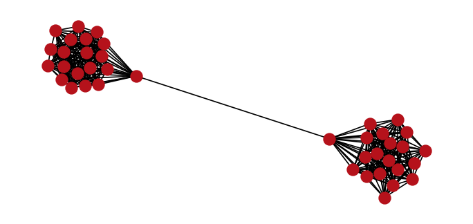
Fig. 26 A barbell graph on 40 vertices, after 30 randomly chosen edges have been removed from within its two clusters.

Computing the graph Laplacian

Graph kernels use the Laplacian matrix \(L\) to quantify the smoothness of a signal (or function) on a graph

(1)\[ L=D-A, \]

where \(D\) is the diagonal degree matrix containing each vertices’ degree and \(A\) is the adjacency matrix that has an \((i,j)^{\text{th}}\) entry of 1 if \(v_i, v_j\) are connected and 0 otherwise. Networkx gives us an easy way to compute this.

L = nx.laplacian_matrix(G).toarray()

glue("graph-kernels-num-edges", f"{G.number_of_edges()}", display=False)

Simulating a signal on the graph

Our task is to construct a Gaussian process \(f(\cdot)\) that maps from the graph’s vertex set \(V\) onto the real line. To that end, we begin by simulating a signal on the graph’s vertices that we will go on to try and predict. We use a single draw from a Gaussian process prior (Prior) to draw our response values \(\boldsymbol{y}\) where we hardcode parameter values. The prior’s covariance is supplied by GraphKernel, which takes the graph Laplacian in place of the usual Euclidean distance. The corresponding input value set for this model, denoted \(\boldsymbol{x}\), is the index set of the graph’s vertices.

x = jnp.arange(G.number_of_nodes()).reshape(-1, 1)

true_kernel = gpx.kernels.GraphKernel(
    laplacian=L,
    lengthscale=2.3,
    variance=3.2,
    smoothness=6.1,
)
prior = gpx.gps.Prior(mean_function=gpx.mean_functions.Zero(), kernel=true_kernel)

fx = prior(x)
y = fx.sample(key=key, sample_shape=(1,)).reshape(-1, 1)

D = gpx.Dataset(X=x, y=y)

/home/runner/work/GPJax/GPJax/.venv/lib/python3.11/site-packages/jaxtyping/_decorator.py:465: UserWarning: X is not of type float64. Got X.dtype=int64. This may lead to numerical instability. 
  out = fn(*args, **kwargs)

We can visualise this signal in Fig. 27.

nx.draw(G, pos, node_color=y, with_labels=False, alpha=0.5)

vmin, vmax = y.min(), y.max()
sm = plt.cm.ScalarMappable(
    cmap=plt.cm.inferno, norm=plt.Normalize(vmin=vmin, vmax=vmax)
)
sm.set_array([])
ax = plt.gca()
cbar = plt.colorbar(sm, ax=ax)
plt.show()

/home/runner/work/GPJax/GPJax/.venv/lib/python3.11/site-packages/IPython/core/pylabtools.py:170: UserWarning: There are no gridspecs with layoutgrids. Possibly did not call parent GridSpec with the "figure" keyword
  fig.canvas.print_figure(bytes_io, **kw)

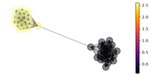
Fig. 27 A single draw from the graph Matern prior, with each vertex coloured by its simulated response value.

Constructing a graph Gaussian process

With our dataset created, we proceed to define our posterior Gaussian process and optimise the model’s hyperparameters. Whilst our underlying space is the graph’s vertex set and is therefore non-Euclidean, our likelihood is still Gaussian and the model is still conjugate. For this reason, we simply perform gradient descent on the GP’s marginal log-likelihood term (conjugate_mll) as in the regression notebook. We do this using the L-BFGS-B optimiser exposed by fit_scipy.

likelihood = gpx.likelihoods.Gaussian(num_datapoints=D.n)
kernel = gpx.kernels.GraphKernel(laplacian=L)
prior = gpx.gps.Prior(mean_function=gpx.mean_functions.Zero(), kernel=kernel)
posterior = prior * likelihood

For researchers and the curious reader, GPJax provides the ability to print the bibtex citation for objects such as the graph kernel through the cite() function.

print(gpx.cite(kernel))

@inproceedings{borovitskiy2021matern,
authors = {Borovitskiy, Viacheslav and Azangulov, Iskander and Terenin, Alexander and Mostowsky, Peter and Deisenroth, Marc and Durrande, Nicolas},
title = {Matérn Gaussian Processes on Graphs},
year = {2021},
booktitle = {International Conference on Artificial Intelligence and Statistics},
}

With a posterior defined, we can now optimise the model’s hyperparameters.

opt_posterior, training_history = gpx.fit_scipy(
    model=posterior,
    objective=lambda p, d: -gpx.objectives.conjugate_mll(p, d),
    train_data=D,
)

         Current function value: -113.647111
         Iterations: 91
         Function evaluations: 132
         Gradient evaluations: 121

/home/runner/work/GPJax/GPJax/.venv/lib/python3.11/site-packages/scipy/optimize/_minimize.py:779: OptimizeWarning: Desired error not necessarily achieved due to precision loss.
  res = _minimize_bfgs(fun, x0, args, jac, callback, **options)

Making predictions

Having optimised our hyperparameters, we can now make predictions on the graph. Though we haven’t defined a training and testing dataset here, we’ll simply query the predictive posterior for the full graph to compare the root-mean-squared error (RMSE) of the model for the initialised parameters vs the optimised set.

initial_dist = likelihood(posterior(x, D))
predictive_dist = opt_posterior.likelihood(opt_posterior(x, D))

initial_mean = initial_dist.mean
learned_mean = predictive_dist.mean

rmse = lambda ytrue, ypred: jnp.sum(jnp.sqrt(jnp.square(ytrue - ypred)))

initial_rmse = jnp.sum(jnp.sqrt(jnp.square(y.squeeze() - initial_mean)))
learned_rmse = jnp.sum(jnp.sqrt(jnp.square(y.squeeze() - learned_mean)))
print(
    f"RMSE with initial parameters: {initial_rmse: .2f}\nRMSE with learned parameters:"
    f" {learned_rmse: .2f}"
)

RMSE with initial parameters:  7.53
RMSE with learned parameters:  0.20

We can also plot the source of error in our model’s predictions on the graph in Fig. 28.

error = jnp.abs(learned_mean - y.squeeze())

nx.draw(G, pos, node_color=error, with_labels=False, alpha=0.5)

vmin, vmax = error.min(), error.max()
sm = plt.cm.ScalarMappable(
    cmap=plt.cm.inferno, norm=plt.Normalize(vmin=vmin, vmax=vmax)
)
ax = plt.gca()
cbar = plt.colorbar(sm, ax=ax)
plt.show()

/home/runner/work/GPJax/GPJax/.venv/lib/python3.11/site-packages/IPython/core/pylabtools.py:170: UserWarning: There are no gridspecs with layoutgrids. Possibly did not call parent GridSpec with the "figure" keyword
  fig.canvas.print_figure(bytes_io, **kw)

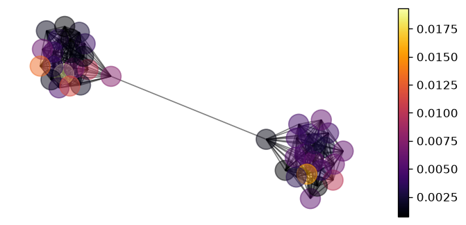
Fig. 28 Absolute error between the optimised posterior mean and the simulated signal at each vertex of the graph.

Reassuringly, our model seems to provide equally good predictions in each cluster.

System configuration

%reload_ext watermark
%watermark -n -u -v -iv -w -a 'Thomas Pinder'

Author: Thomas Pinder

Last updated: Sat, 01 Aug 2026

Python implementation: CPython
Python version       : 3.11.15
IPython version      : 9.15.0

gpjax     : 0.18.0
jax       : 0.10.2
jaxtyping : 0.3.11
matplotlib: 3.11.1
myst_nb   : 1.4.0
networkx  : 3.6.1

Watermark: 2.6.0