Joint Inference with Numpyro#
Download this notebook: numpyro_integration.ipynb
In this notebook, we demonstrate how to use Numpyro to perform fully Bayesian inference over the hyperparameters of a Gaussian process model. We will look at a scenario where we have a structured mean function in the form of a linear model, and a GP capturing the residuals. We will infer the parameters of both the linear model and the GP jointly.
from utils import use_mpl_style
import gpjax as gpx
from jax import config
import jax.numpy as jnp
import jax.random as jr
import matplotlib as mpl
import matplotlib.pyplot as plt
import numpyro
import numpyro.distributions as dist
from numpyro.infer import (
    MCMC,
    NUTS,
    Predictive,
)

config.update("jax_enable_x64", True)

use_mpl_style()
cols = mpl.rcParams["axes.prop_cycle"].by_key()["color"]

key = jr.key(123)
keys = jr.split(key, 4)
Data Generation#
We generate a synthetic dataset that consists of a linear trend together with a locally periodic residual signal whose amplitude varies over time, an additional high-frequency component, and a local bump (Fig. 46). This data generating process is purposefully designed to illustrate the benefit of incorporating a Gaussian process into a larger Bayesian model; however, such structures are common.
N = 200

x = jnp.sort(jr.uniform(keys[0], shape=(N, 1), minval=0.0, maxval=10.0), axis=0)

# True parameters for the linear trend
true_slope = 0.45
true_intercept = 1.5

# Structured residual signal captured by the GP
slow_period = 6.0
fast_period = 0.8
amplitude_envelope = 1.0 + 0.5 * jnp.sin(2 * jnp.pi * x / slow_period)
modulated_periodic = amplitude_envelope * jnp.sin(2 * jnp.pi * x / fast_period)
high_frequency_component = 0.3 * jnp.cos(2 * jnp.pi * x / 0.35)
localised_bump = 1.2 * jnp.exp(-0.5 * ((x - 7.0) / 0.45) ** 2)

linear_trend = true_slope * x + true_intercept
residual_signal = modulated_periodic + high_frequency_component + localised_bump
signal = linear_trend + residual_signal

# Observations with homoscedastic noise
observation_noise = 0.7
y = signal + observation_noise * jr.normal(keys[1], shape=x.shape)

D = gpx.Dataset(X=x, y=y)

fig, ax = plt.subplots()
ax.plot(x, y, "o", label="Observations", color=cols[0])
ax.plot(x, signal, "--", label="True Signal", color=cols[1])
ax.legend()
plt.show()
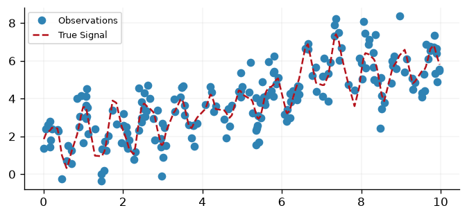
Fig. 46 Synthetic observations drawn around a true signal that combines a linear trend with a locally periodic residual, a high-frequency component and a localised bump.#
Model Definition#
We define a GP model with a zero mean function, as we will handle the linear
trend explicitly in the Numpyro model. Naturally, one could parameterise the GP with a
linear mean function; however, this design is purely pedagogical. For the kernel, we specify a
product of a Periodic kernel and an
RBF kernel. This choice reflects our prior knowledge that
the signal is locally periodic. For a more in-depth look at how complex kernels can be designed,
see our
Introduction to Kernels
notebook.
We see in the below that priors are specified on the parameters’ constrained space. For
example, the lengthscale parameter must be strictly positive and, therefore, a unit-Gaussian
would be a poor choice of prior. Instead, we opt for the log-Gaussian as the prior distribution
as its support matches that of our lengthscale parameter. Priors are standard
NumPyro distributions sampled directly
inside the model function with numpyro.sample.
Priors are defined as NumPyro distributions and sampled directly inside the model function below. GPJax parameter constructors accept raw JAX arrays from numpyro.sample, so no special registration step is needed.
We’ll construct the Gaussian process inside the NumPyro model function, passing sampled hyperparameters directly to the GPJax constructors. For a deeper look at how GP construction works, see our Regression notebook.
Joint Inference Loop#
We define a NumPyro model that samples all parameters directly using
numpyro.sample, builds the GPJax
ConjugatePosterior from those samples, and
scores it with the conjugate marginal log-likelihood
(conjugate_mll) via numpyro.factor.
No special registration step is needed – GPJax constructors accept raw
JAX arrays returned by numpyro.sample.
def model(X, Y, X_new=None):
    slope = numpyro.sample("slope", dist.Normal(0.0, 2.0))
    intercept = numpyro.sample("intercept", dist.Normal(0.0, 2.0))
    linear_component = slope * X + intercept

    residuals = Y - linear_component

    lengthscale = numpyro.sample("lengthscale", dist.LogNormal(0.0, 1.0))
    variance = numpyro.sample("variance", dist.LogNormal(0.0, 1.0))
    period = numpyro.sample("period", dist.LogNormal(0.0, 0.5))
    obs_noise = numpyro.sample("obs_noise", dist.LogNormal(0.0, 1.0))

    stationary_component = gpx.kernels.RBF(lengthscale=lengthscale, variance=variance)
    periodic_component = gpx.kernels.Periodic(lengthscale=lengthscale, period=period)
    kernel = stationary_component * periodic_component

    meanf = gpx.mean_functions.Constant()
    prior = gpx.gps.Prior(mean_function=meanf, kernel=kernel)
    likelihood = gpx.likelihoods.Gaussian(num_datapoints=N, obs_stddev=obs_noise)
    posterior = prior * likelihood

    D_resid = gpx.Dataset(X=X, y=residuals)
    mll = gpx.objectives.conjugate_mll(posterior, D_resid)

    numpyro.factor("gp_log_lik", mll)

    if X_new is not None:
        latent_dist = posterior.predict(X_new, train_data=D_resid)
        f_new = numpyro.sample("f_new", latent_dist)
        f_new = f_new.reshape((-1, 1))

        y_noise = numpyro.sample(
            "y_noise",
            dist.Normal(0.0, obs_noise).expand(f_new.shape).to_event(f_new.ndim),
        )

        total_prediction = slope * X_new + intercept + f_new + y_noise
        numpyro.deterministic("y_pred", total_prediction)
        return total_prediction
Inspecting the model and its priors#
Before running inference it is helpful to lay out the model’s parameters alongside the
priors we placed on them. Because the priors are sampled by name inside model and
passed into the GPJax constructors, they are not stored on the parameter objects – so
gpx.summarise cannot infer them automatically. We can still
display them by passing a priors mapping keyed by each parameter’s name (the entries in
the Parameter column; call gpx.summarise(example_posterior) without the mapping to
discover them).
The parameter values shown are placeholders – they are resampled from these priors at
every step of MCMC.
example_kernel = gpx.kernels.RBF(lengthscale=1.0, variance=1.0) * gpx.kernels.Periodic(
    lengthscale=1.0, period=1.0
)
example_posterior = gpx.gps.Prior(
    mean_function=gpx.mean_functions.Constant(), kernel=example_kernel
) * gpx.likelihoods.Gaussian(num_datapoints=N, obs_stddev=1.0)

parameter_priors = {
    "prior.kernel.kernels[0].lengthscale": dist.LogNormal(0.0, 1.0),
    "prior.kernel.kernels[0].variance": dist.LogNormal(0.0, 1.0),
    "prior.kernel.kernels[1].lengthscale": dist.LogNormal(0.0, 1.0),
    "prior.kernel.kernels[1].period": dist.LogNormal(0.0, 0.5),
    "likelihood.obs_stddev": dist.LogNormal(0.0, 1.0),
}

gpx.summarise(example_posterior, priors=parameter_priors)
ConjugatePosterior
╭───────────────────────┬─────────────────┬───────┬──────────┬────────────────────────┬───────────┬───────┬───────╮
│ Parameter             │ Class           │ Value │ Bijector │ Prior                  │ Trainable │ Shape │ Dtype │
├───────────────────────┼─────────────────┼───────┼──────────┼────────────────────────┼───────────┼───────┼───────┤
│ prior.kernel.kernels[ │ PositiveReal    │ 1     │ Softplus │ LogNormal(loc=0,       │ yes       │ ()    │ f64   │
│ 0].lengthscale        │                 │       │          │ scale=1)               │           │       │       │
│ prior.kernel.kernels[ │ NonNegativeReal │ 1     │ Softplus │ LogNormal(loc=0,       │ yes       │ ()    │ f64   │
│ 0].variance           │                 │       │          │ scale=1)               │           │       │       │
│ prior.kernel.kernels[ │ PositiveReal    │ 1     │ Softplus │ LogNormal(loc=0,       │ yes       │ ()    │ f64   │
│ 1].lengthscale        │                 │       │          │ scale=1)               │           │       │       │
│ prior.kernel.kernels[ │ NonNegativeReal │ 1     │ Softplus │ -                      │ yes       │ ()    │ f64   │
│ 1].variance           │                 │       │          │                        │           │       │       │
│ prior.kernel.kernels[ │ PositiveReal    │ 1     │ Softplus │ LogNormal(loc=0,       │ yes       │ ()    │ f64   │
│ 1].period             │                 │       │          │ scale=0.5)             │           │       │       │
│ prior.mean_function.c │ Array           │ 0     │ Identity │ -                      │ yes       │ ()    │ f64   │
│ onstant               │                 │       │          │                        │           │       │       │
│ likelihood.obs_stddev │ NonNegativeReal │ 1     │ Softplus │ LogNormal(loc=0,       │ yes       │ ()    │ f64   │
│                       │                 │       │          │ scale=1)               │           │       │       │
╰───────────────────────┴─────────────────┴───────┴──────────┴────────────────────────┴───────────┴───────┴───────╯
7 parameters, 7 trainable
Running MCMC#
Using Numpyro’s NUTS sampler, we can now draw samples
from the posterior. To ensure
our documentation can be quickly built, we limit the number of samples and the length
of the burn-in phase below. However, in practice, one should draw more samples from
multiple chains using the num_chains argument in the MCMC constructor.
nuts_kernel = NUTS(model)
# In practice, one should run more samples from multiple chains.
mcmc = MCMC(
    nuts_kernel,
    num_warmup=50 if ci else 750,
    num_samples=50 if ci else 500,
)
mcmc.run(keys[2], x, y)
mcmc.print_summary()
                   mean       std    median      5.0%     95.0%     n_eff     r_hat
    intercept      1.17      1.88      1.75     -1.58      3.66      4.92      1.08
  lengthscale      2.75      0.66      2.78      1.70      3.54     17.47      0.99
    obs_noise      0.80      0.05      0.81      0.73      0.88     20.72      1.01
       period      0.80      0.02      0.80      0.77      0.82     36.86      1.00
        slope      0.33      0.28      0.42     -0.18      0.66      5.03      1.10
     variance      7.93      3.62      7.32      3.93     15.64     10.58      1.01

Number of divergences: 1
Analysis and Plotting#
Having obtained samples from the posterior, we now evaluate the predictive posterior
at the test sites. In our
Poisson Regression, this
process is done manually. However, by virtue of using Numpyro here, we may instead
use Numpyro’s Predictive object to handle this
process for us. Once samples are
drawn from the predictive posterior distribution, we may evaluate the mean and 95%
credible interval and compare our model’s predictions to the underlying data
(Fig. 47).
samples = mcmc.get_samples()
predictive = Predictive(
    model,
    posterior_samples=samples,
    return_sites=["y_pred"],
)

x_test = jnp.linspace(-0.5, 10.5, 200).reshape(-1, 1)
predictions = predictive(keys[3], x, y, X_new=x_test)
y_pred = predictions["y_pred"]

mean_prediction = jnp.mean(y_pred, axis=0)
lower, upper = jnp.percentile(y_pred, jnp.array([2.5, 97.5]), axis=0)

fig, ax = plt.subplots()
ax.scatter(x, y, alpha=0.5, label="Observations", color=cols[0])
ax.plot(x, signal, "--", label="True Signal", color=cols[0])

ax.plot(x_test, mean_prediction, "-", label="Posterior Mean", color=cols[1])
ax.fill_between(
    x_test.flatten(),
    lower.flatten(),
    upper.flatten(),
    color=cols[1],
    alpha=0.2,
    label="95% Credible Interval",
)
ax.legend()
plt.show()
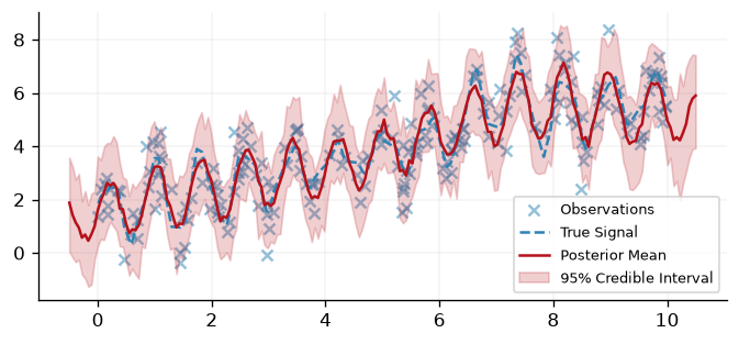
Fig. 47 Posterior predictive mean and 95% credible interval obtained from the NUTS samples, shown against the observations and the true signal.#
Conclusions#
This concludes our introduction to the integration of GPJax with Numpyro. The presentation given here is designed to best illustrate how the two libraries integrate. For a closer look at the more complex models that one may build by integrating Numpyro and GPJax, see our Spatial Semi-Linear Model notebook.
System configuration#
%load_ext watermark
%watermark -n -u -v -iv -w -a "Thomas Pinder"
Author: Thomas Pinder

Last updated: Sat, 01 Aug 2026

Python implementation: CPython
Python version       : 3.11.15
IPython version      : 9.15.0

gpjax     : 0.18.0
jax       : 0.10.2
matplotlib: 3.11.1
numpyro   : 0.21.0

Watermark: 2.6.0