Sparse Gaussian Process Regression

Download this notebook: collapsed_vi.ipynb

In this notebook we consider sparse Gaussian process regression (SGPR) [Titsias, 2009]. This is a solution for medium to large-scale conjugate regression problems. In order to arrive at a computationally tractable method, the approximate posterior is parameterized via a set of \(m\) pseudo-points \(\boldsymbol{z}\). Critically, the approach leads to \(\mathcal{O}(nm^2)\) complexity for approximate maximum likelihood learning and \(O(m^2)\) per test point for prediction. The bound used here is collapsed: the variational parameters are solved for analytically, which requires a conjugate (Gaussian) likelihood and a pass over the full dataset. Lifting either restriction — a non-Gaussian likelihood, or mini-batched optimisation — calls for the uncollapsed bound of the sparse stochastic variational inference notebook.

# Enable Float64 for more stable matrix inversions.
from utils import use_mpl_style
from jax import (
    config,
    jit,
)
import jax.numpy as jnp
import jax.random as jr
from jaxtyping import install_import_hook
import matplotlib as mpl
import matplotlib.pyplot as plt
import optax as ox

config.update("jax_enable_x64", True)


with install_import_hook("gpjax", "beartype.beartype"):
    import gpjax as gpx


# set the default style for plotting
use_mpl_style()

key = jr.key(42)

cols = mpl.rcParams["axes.prop_cycle"].by_key()["color"]

Dataset

With the necessary modules imported, we simulate a dataset \(\mathcal{D} = (\boldsymbol{x}, \boldsymbol{y}) = \{(x_i, y_i)\}_{i=1}^{500}\) with inputs \(\boldsymbol{x}\) sampled uniformly on \((-3., 3)\) and corresponding independent noisy outputs

(1)\[ \boldsymbol{y} \sim \mathcal{N} \left(\sin(7\boldsymbol{x}) + x \cos(2 \boldsymbol{x}), \textbf{I} * 0.5^2 \right). \]

We store our data \(\mathcal{D}\) as a GPJax Dataset and create test inputs and labels for later.

n = 2500
noise = 0.5

key, subkey = jr.split(key)
x = jr.uniform(key=key, minval=-3.0, maxval=3.0, shape=(n,)).reshape(-1, 1)
f = lambda x: jnp.sin(2 * x) + x * jnp.cos(5 * x)
signal = f(x)
y = signal + jr.normal(subkey, shape=signal.shape) * noise

D = gpx.Dataset(X=x, y=y)

xtest = jnp.linspace(-3.1, 3.1, 500).reshape(-1, 1)
ytest = f(xtest)

To better understand what we have simulated, we plot both the underlying latent function and the observed data that is subject to Gaussian noise. We also plot an initial set of inducing points over the space.

n_inducing = 50
z = jnp.linspace(-3.0, 3.0, n_inducing).reshape(-1, 1)

fig, ax = plt.subplots()
ax.scatter(x, y, alpha=0.25, label="Observations", color=cols[0])
ax.plot(xtest, ytest, label="Latent function", linewidth=2, color=cols[1])
ax.vlines(
    x=z,
    ymin=y.min(),
    ymax=y.max(),
    alpha=0.3,
    linewidth=0.5,
    label="Inducing point",
    color=cols[2],
)
ax.legend(loc="best")
plt.show()

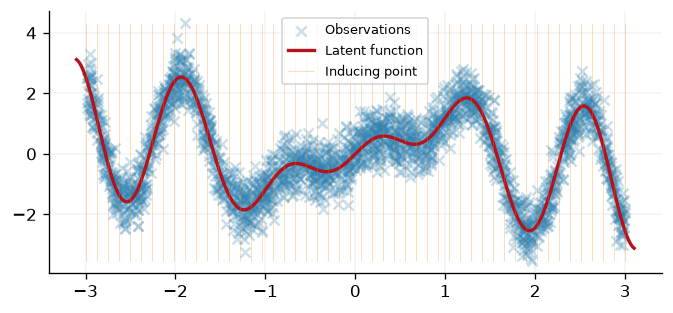
Fig. 12 The simulated observations, the latent function that generated them, and the evenly spaced inducing points used to initialise the sparse model.

Next we define the true posterior model for the data - note that whilst we can define this, it is intractable to evaluate.

meanf = gpx.mean_functions.Constant()
kernel = gpx.kernels.RBF()  # 1-dimensional inputs
likelihood = gpx.likelihoods.Gaussian(num_datapoints=D.n)
prior = gpx.gps.Prior(mean_function=meanf, kernel=kernel)
posterior = prior * likelihood

We now define the SGPR model through CollapsedVariationalGaussian. Through a set of inducing points \(\boldsymbol{z}\) this object builds an approximation to the true posterior distribution. Consequently, we pass the true posterior and initial inducing points into the constructor as arguments.

q = gpx.variational_families.CollapsedVariationalGaussian(
    posterior=posterior, inducing_inputs=z
)

We now train our model akin to a Gaussian process regression model via the fit abstraction. Unlike the regression example given in the conjugate regression notebook, the inducing locations that induce our variational posterior distribution are now part of the model’s parameters. Using a gradient-based optimiser, we can then optimise their location such that the evidence lower bound is maximised.

# Use the enhanced fit API with trainable parameter filtering
opt_posterior, history = gpx.fit(
    model=q,
    # we want want to minimize the *negative* ELBO
    objective=lambda p, d: -gpx.objectives.collapsed_elbo(p, d),
    train_data=D,
    optim=ox.adamw(learning_rate=1e-2),
    num_iters=500,
    key=key,
)

fig, ax = plt.subplots()
ax.plot(history, color=cols[1])
ax.set(xlabel="Training iterate", ylabel="ELBO")

[Text(0.5, 0, 'Training iterate'), Text(0, 0.5, 'ELBO')]

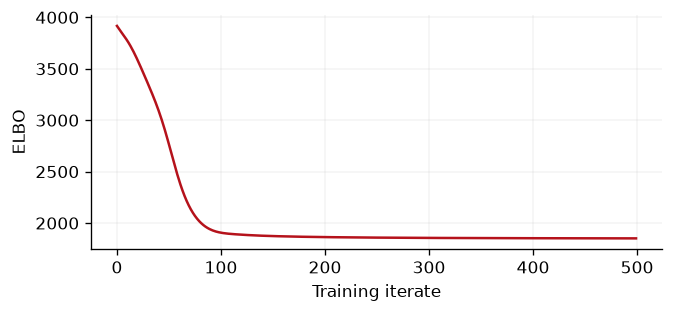
Fig. 13 shows predictions of our model with the learned inducing points overlaid in grey.

latent_dist = opt_posterior(xtest, train_data=D)
predictive_dist = opt_posterior.posterior.likelihood(latent_dist)

inducing_points = opt_posterior.inducing_inputs.unwrap()

samples = latent_dist.sample(key=key, sample_shape=(20,))

predictive_mean = predictive_dist.mean
predictive_std = jnp.sqrt(predictive_dist.variance)

fig, ax = plt.subplots()

ax.plot(x, y, "x", label="Observations", color=cols[0], alpha=0.1)
ax.plot(
    xtest,
    ytest,
    label="Latent function",
    color=cols[1],
    linestyle="-",
    linewidth=1,
)
ax.plot(xtest, predictive_mean, label="Predictive mean", color=cols[1])

ax.fill_between(
    xtest.squeeze(),
    predictive_mean - 2 * predictive_std,
    predictive_mean + 2 * predictive_std,
    alpha=0.2,
    color=cols[1],
    label="Two sigma",
)
ax.plot(
    xtest,
    predictive_mean - 2 * predictive_std,
    color=cols[1],
    linestyle="--",
    linewidth=0.5,
)
ax.plot(
    xtest,
    predictive_mean + 2 * predictive_std,
    color=cols[1],
    linestyle="--",
    linewidth=0.5,
)


ax.vlines(
    x=inducing_points,
    ymin=ytest.min(),
    ymax=ytest.max(),
    alpha=0.3,
    linewidth=0.5,
    label="Inducing point",
    color=cols[2],
)
ax.legend()
ax.set(xlabel=r"$x$", ylabel=r"$f(x)$")
plt.show()

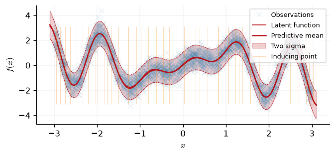
Fig. 13 Predictive mean and two-standard-deviation band of the sparse posterior, shown against the observations and the latent function, with the optimised inducing point locations overlaid.

Runtime comparison

Given the size of the data being considered here, inference in a GP with a full-rank covariance matrix is possible, albeit quite slow — the cubic cost described in the sharp bits. We can therefore compare the speedup that we get from using the above sparse approximation with corresponding bound on the marginal log-likelihood against the marginal log-likelihood in the full model.

full_rank_model = gpx.gps.Prior(
    mean_function=gpx.mean_functions.Zero(), kernel=gpx.kernels.RBF()
) * gpx.likelihoods.Gaussian(num_datapoints=D.n)
nmll = jit(lambda: -gpx.objectives.conjugate_mll(full_rank_model, D))
%timeit nmll().block_until_ready()

89.3 ms ± 2 ms per loop (mean ± std. dev. of 7 runs, 10 loops each)

nelbo = jit(lambda: -gpx.objectives.collapsed_elbo(q, D))
%timeit nelbo().block_until_ready()

1.52 ms ± 751 μs per loop (mean ± std. dev. of 7 runs, 1 loop each)

As we can see, the sparse approximation given here is much faster when compared against a full-rank model.

System configuration

%reload_ext watermark
%watermark -n -u -v -iv -w -a 'Daniel Dodd'

Author: Daniel Dodd

Last updated: Sat, 01 Aug 2026

Python implementation: CPython
Python version       : 3.11.15
IPython version      : 9.15.0

gpjax     : 0.18.0
jax       : 0.10.2
jaxtyping : 0.3.11
matplotlib: 3.11.1
optax     : 0.2.8

Watermark: 2.6.0